Processing geospatial data with QGIS
QGIS is a free and open-source geographic information system that can be used to process data that can support the land use classification process. Where existing land use or land cover data is available in a spatial format, users can convert vector (points, line, polygons) and raster (images) data into KML files that can be viewed in Google Earth during a land use classification with Collect Earth. KML files are also compatible with Google Fusion Tables and can be imported into Google Earth Engine.
Click on the steps below to view details.
Visit the Open Source Geospatial Foundation website to download QGIS along with many supplementary packages that can be utilized through the software. Download the OSGeo4W installer for 32bit of 64bit.
While running the installer, select the Express Install option and choose the packages to install. Once the installation is complete, you can launch the program from the Start Menu.
Click on the vector icon in the left-hand panel to add a vector layer to your data frame in QGIS.
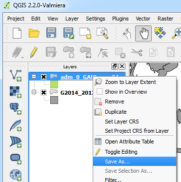
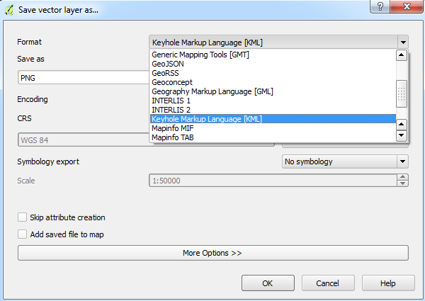
Right-click on the layer and select Save as. Select the KML format, which can be viewed in Google Earth while assessing land use with Collect Earth.
This steps below describe how to import maps and images without a spatial reference system directly into Google Earth as image overlays. For other types of raster data (with existing spatial data), use QGIS with a plugin called GEarthViewer to convert rasters into Google Earth overlays through a simple process that retains their geographic positioning. Click here for more information.
Click on the raster icon in the left-hand panel to add a raster layer to your data frame in QGIS. Under the Plugins menu, click on Manage and Install Plugins.
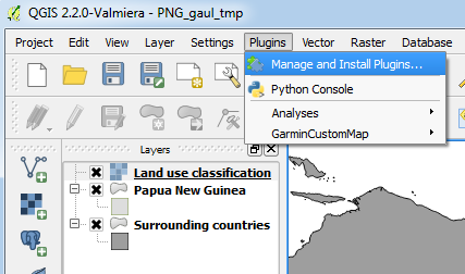
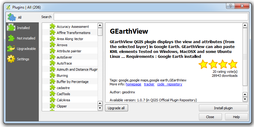
Search for and install a plugin called GEarthView.
Click on the GEarthView icon in the toolbar and select GEarthView from the options below to export a snapshot of your QGIS data frame to Google Earth.
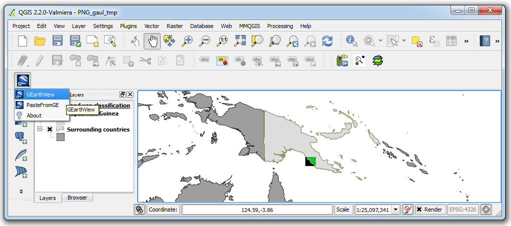
Everything that is visible in QGIS as one overlay. Although vector files can also be exported with this tool, importing vectors as KMLs enables more flexibility in visualization.
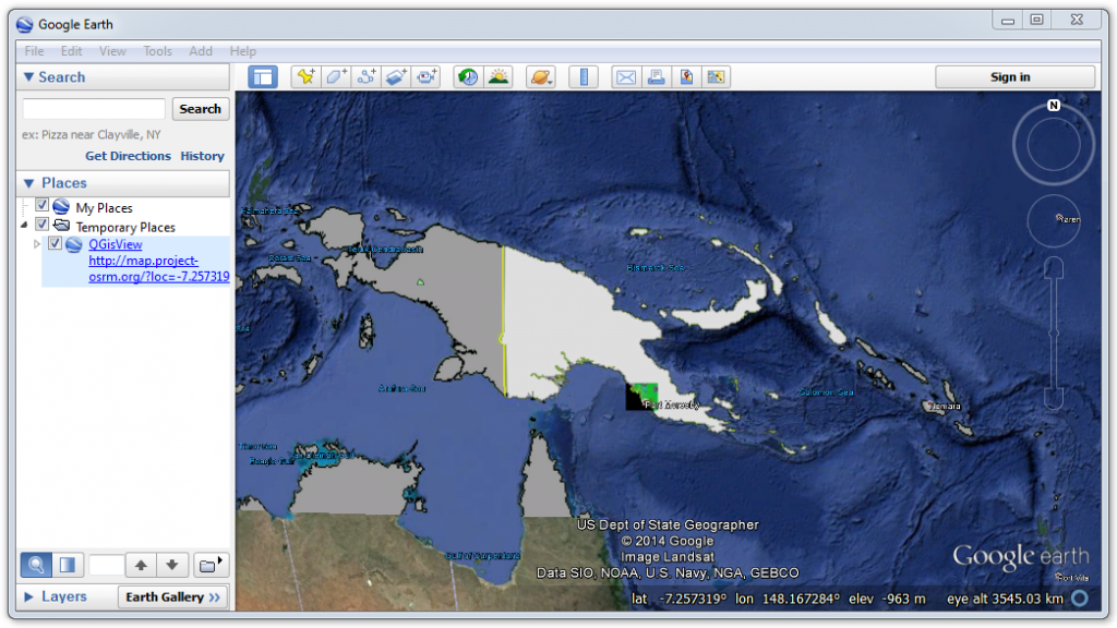
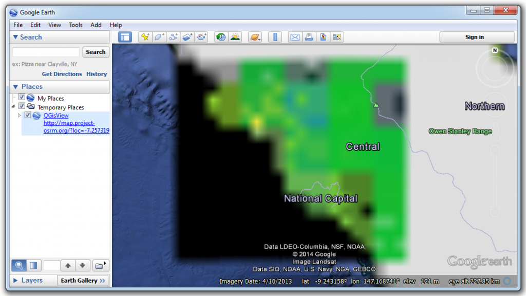
The resolution of rasters will vary based on the scale of the QGIS data frame. This 30m resolution raster is blurry when exported from QGIS at a 1:25,000,000 scale.
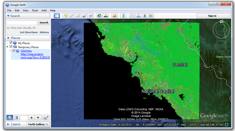
This 30m resolution raster is much clearer when exported from QGIS at a scale of 1:2,000,000.
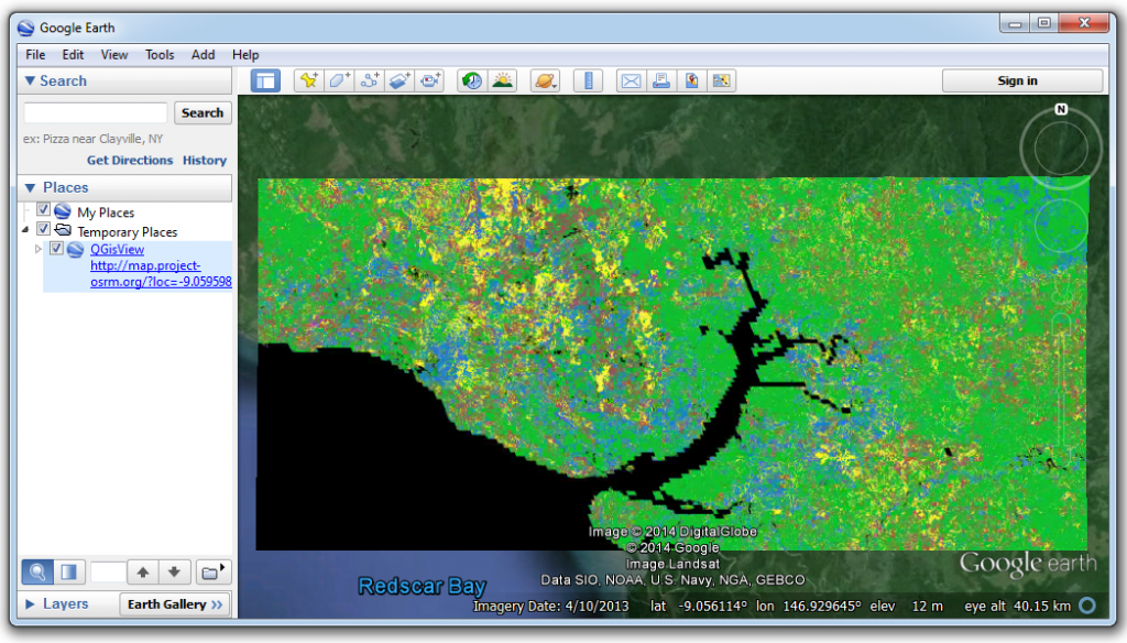
The resolution of the export decreases as the scale in QGIS increases. This section of the raster was exported with QGIS at a scale 1:200,000.
Generating sampling points for Collect Earth – Manual process
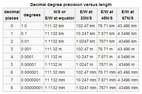
The following section reviews the process for creating a grid in decimal degrees using South Africa as an example. Many countries use a coarse or medium scale 1° x 1° or 0.05° x 0.05° grids. Where specific geographic areas (e.g. small administrative areas or land use strata) with relatively small spatial extents exist, a country may choose to stratify their sampling apply a smaller grid in certain areas.
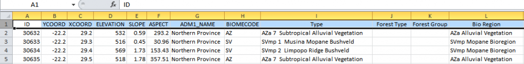
The objective is to create a csv file with six basic columns and attributes required to use the file in Collect Earth: plot ID number, latitude, longitude, elevation, slope and aspect. In some country-specific versions of Collect Earth, additional attributes may also required columns, such as province name, biome code, biome type, forest type, forest group and bioregion. For non-essential attributes, the column can be left blank provided that the column headers for the required attributes are added.
Country boundaries and spatial data for lower administrative levels can be used to define the spatial extent for the grid. A global dataset of administrative boundaries is available on the GADM website . Spatial data can be downloaded in shapefile, KMZ and other formats.
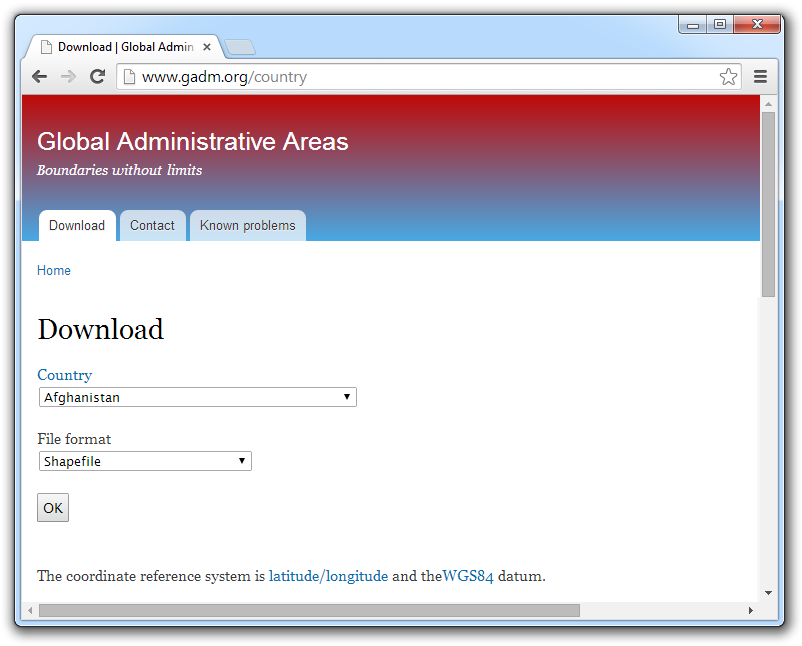
More accurate spatial data may be available from official government agencies. Spatial data of South Africa is provided by the Municipal Demarcation Board.
Open the administrative boundary layer in QGIS. Right click on the layer and select properties. In the left sidebar, click on Metadata, the last option. Check the spatial reference system of the layer. This will determine the units of measurement used for the grid.
This layer for South Africa is in WGS 84 datum with no projection specified. The grid created in WGS 84 will use decimal degrees as its unit of measurement.
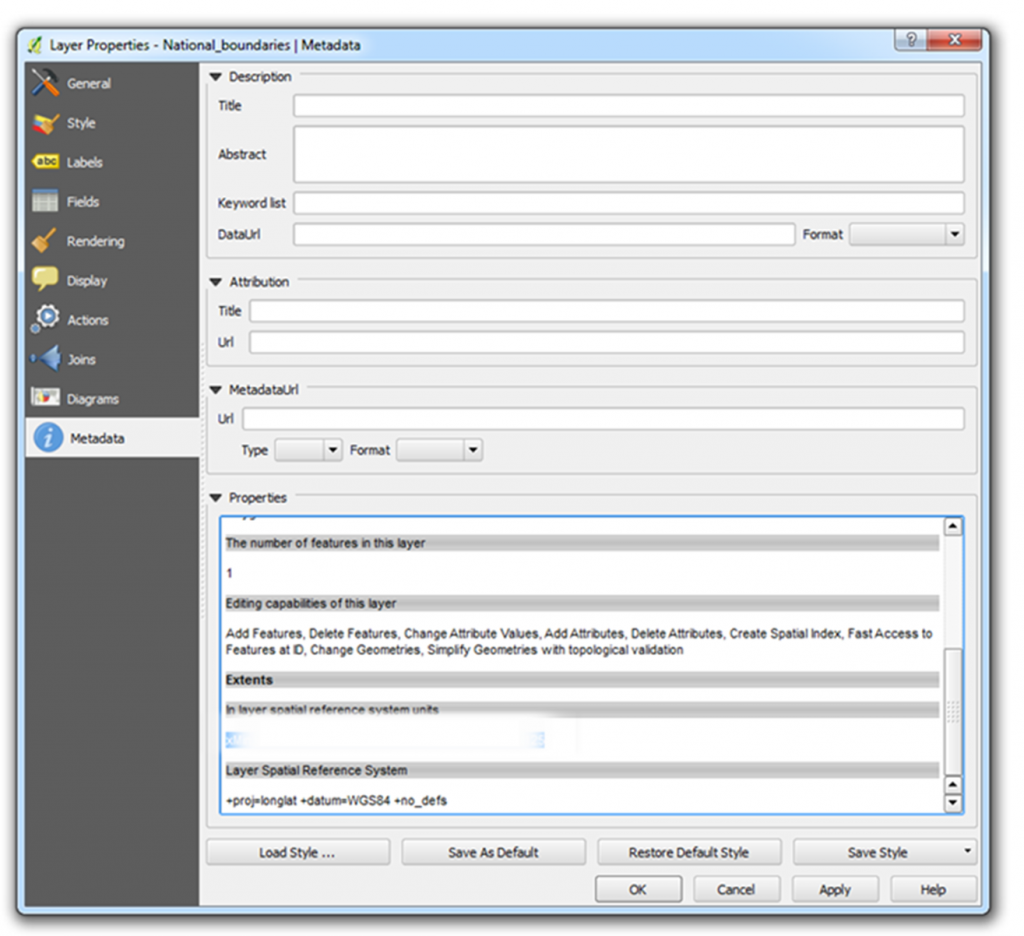
Copy the spatial extent of the layer.
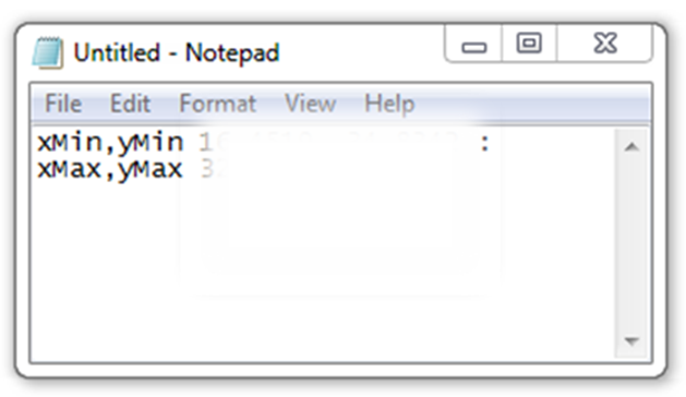
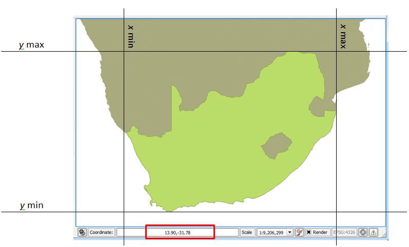
Click cancel to escape the metadata window. Explore the spatial extent in the map frame by moving the mouse over the layer and observing the changes in the coordinates at the bottom of the QGIS window.
It is useful to create a grid with relatively round numbers. A subset of the points may be used for a ground-based forest inventory. Coordinates with one or two decimal places are easier to manually enter into a GPS unit than coordinates with more digits. (However, various software tools exist to transfer spatial data onto GPS units.) To simplify the coordinates of the grid, the spatial extent values will be rounded to whole numbers and manually entered as the spatial extent of the grid.
In the main tool bar, click on Vector, Research Tools and Regular points.
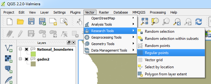
Refer to South Africa’s spatial extent, which you pasted in Notepad. Round the X min and Y min values down, and round X max and Y max values up.
- Specify the desired grid spacing. Here, 0.01 degrees will be the distance between points in the grid.
- Specify the name and location for the new grid, click the box to Add result to canvas and click OK.
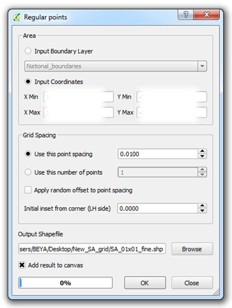
At first glance, the resulting grid appears to be a solid polygon. Zoom in to view the grid more closely.
Measure the distance between the grid points to confirm that the operation has been properly completed. Click on the dropdown arrow beside the ruler icon and select Measure Line.
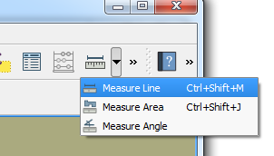
Left click on a grid point to start the line. Right click on an adjacent point to finish the line. Measure the east-west distance instead of the north-south length. The length of the line will be displayed in the Measurement window.
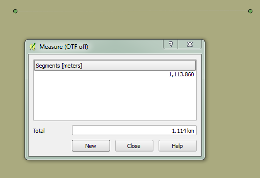
The distance between points is roughly 1.11 km. This is close to what one might expect 0.01° to equal in South Africa, which ranges from 21° to 35° south of the equator. The decimal degree-to-kilometers estimates in the table are explained in more detail on Wikipedia here . In short, the east-west distance of 1° at the equator is equal to the circumference of the earth (40,075 km) divided by 360 degrees: 111.32 km. At other latitudes, the distance will be slightly shorter as the circumference of the earth tapers toward the north and south poles.
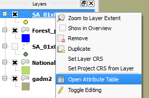
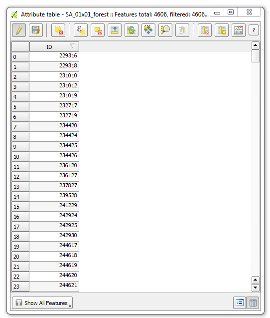
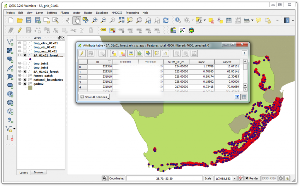
Right click on the grid layer and select Open Attribute Table.
At this point, the table only contains the point IDs. The total number of points has been reduced from 2,379,999 to 4,605.
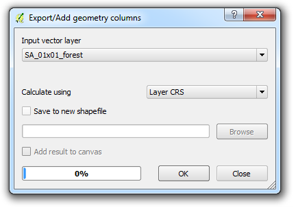
Under the Vector menu, click on Geometry Tools and Export/Add geometry columns.
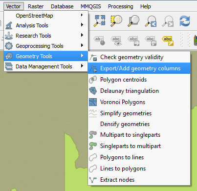
Select the grid layer with points only in the area of interest as the Input vector layer. Click OK.
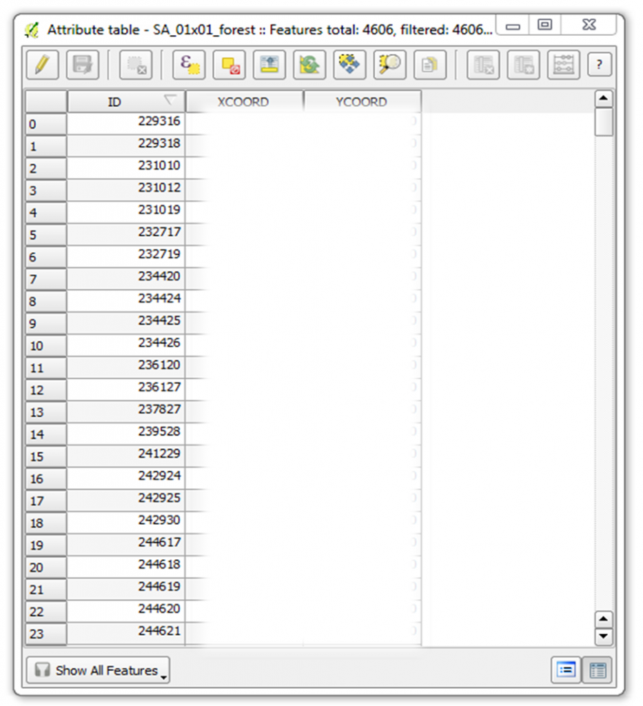
Once the process is complete, right click on the layer and check the data attribute table. Confirm that the X (longitude), Y (latitude) coordinates have been added.
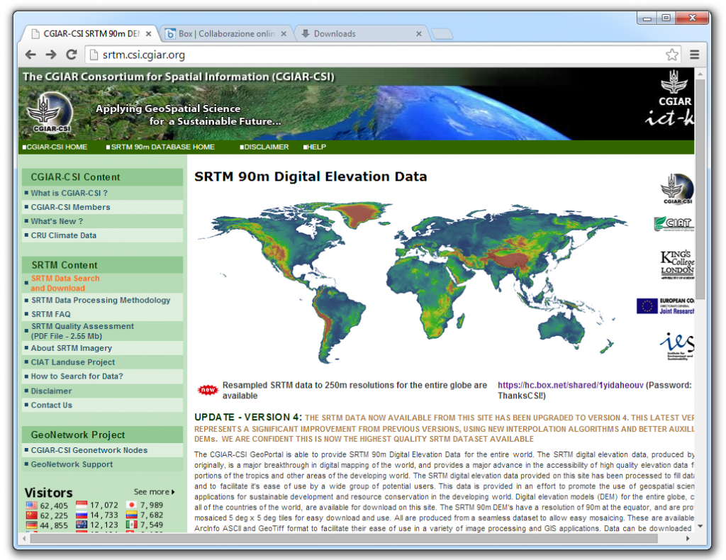
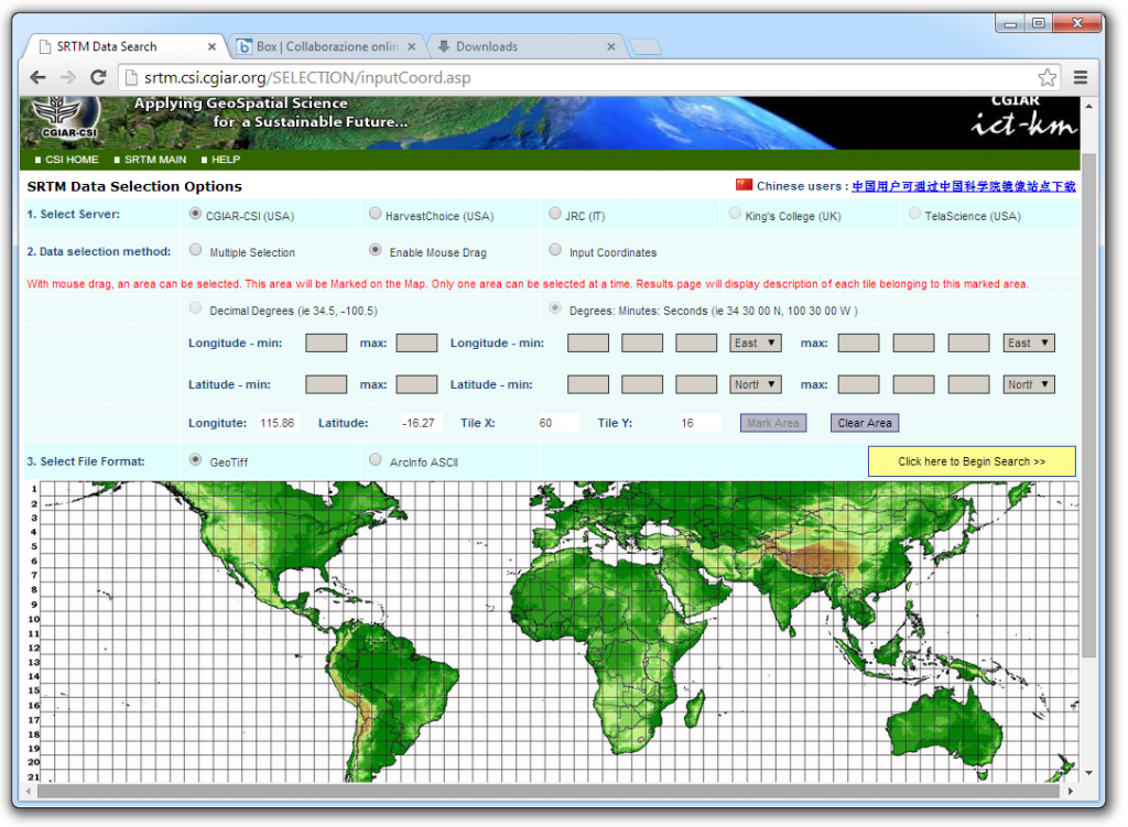
Visit the Consultative Group on International Agricultural Research, Consortium for Spatial Information (CGIAR-CSI) website to download 90m resolution digital elevation data. The data, originally from NASA’s Shuttle Radar Topography Mission, is available in GeoTiff and ArcInfo format. To download only the tiles covering the area of interest, click on the link SRTM Data Search and Download.
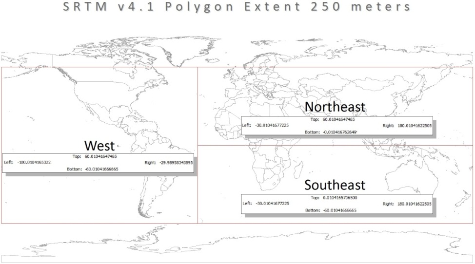
The global dataset can be downloaded by region (West, Northeast and Southeast) by clicking on this link and entering the password listed beside it.
On the SRTM Data Search page, select CGIAR-CSI as the server, enable mouse drag as the data selection method, and choose GeoTiff as the file format. Click and drag the mouse over the relevant tiles. Download your selection.
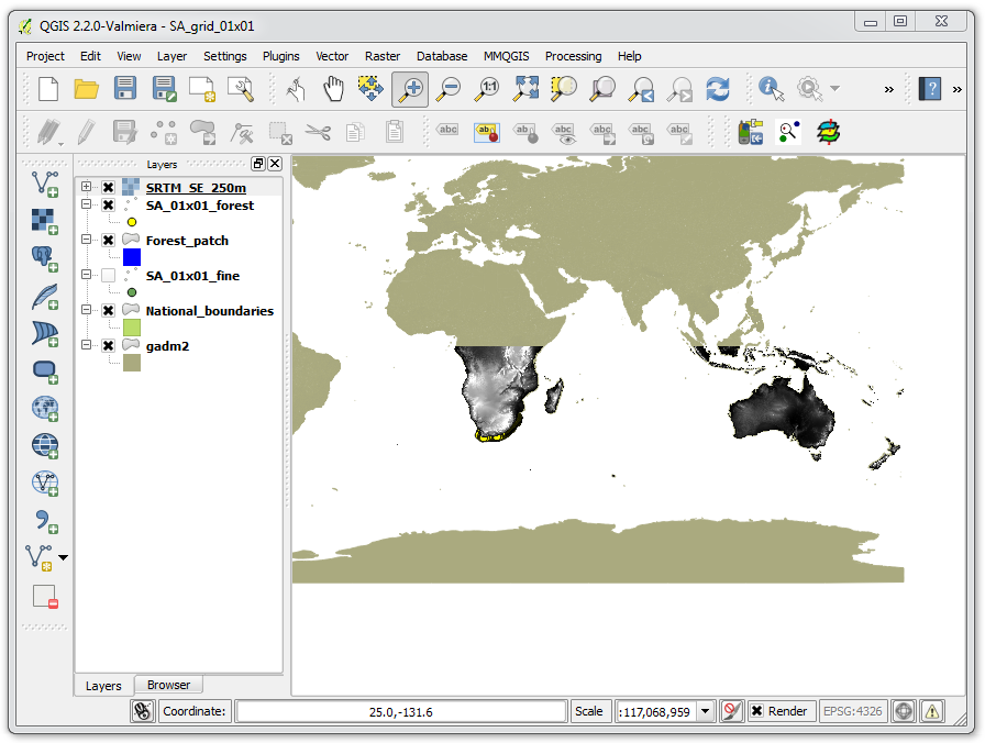
Once the download is complete, load the geotiff in QGIS.
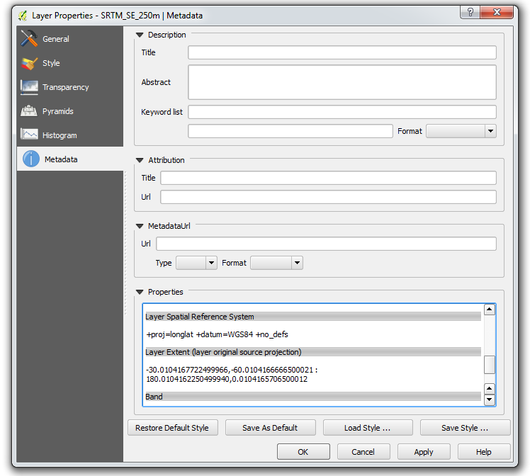
Right click on the layer and review the metadata to confirm that it is in the same projection as the other spatial data you are using.
Under the Raster menu, click on Analysis and DEM (Terrain models).
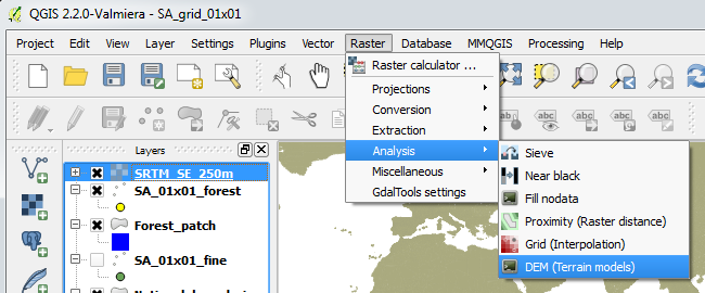
- Input the SRTM digital elevation data.
- Specify the output location and file name.
- Check the box for band and select 1 (there is only one band in the SRTM data).
- Click on the dropdown arrow beside mode and select Slope.
- Type in 111120 as the scale for converting meters to decimal degrees. (For more information on this conversion, visit the GDAL website
- Check the box to load the resulting layer once the process is complete. Then click OK.
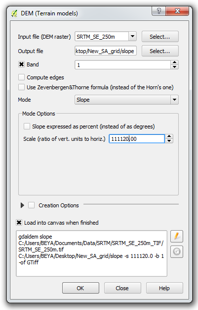
Use the same tool to derive aspect data.
- Input the SRTM digital elevation model data.
- Specify the output location and file name.
- Check the box for band and select 1 (there is only one band in the SRTM data).
- Click on the dropdown arrow beside mode and select Aspect.
- Check the box to return 0 for flat instead of -9999.
- Check the box to load the resulting layer once the process is complete. Then click OK.
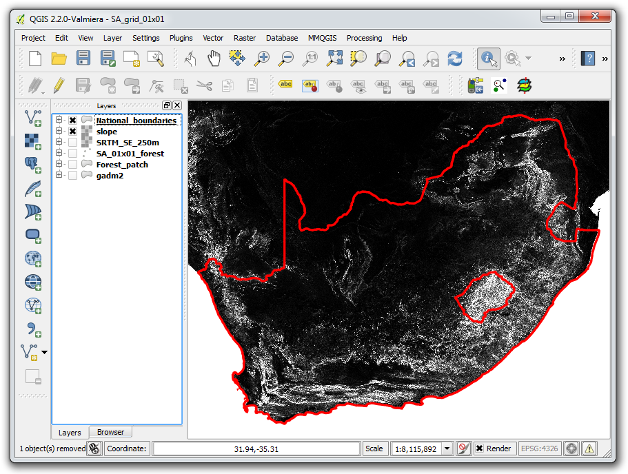
The resulting slope and aspect layers are raster files separate from the original SRTM elevation raster.
There are two parts to this step. In the first part, elevation, slope and aspect data are extracted from the rasters and associated with each point in the forest grid. This results in three separate point files. The second part involves consolidating the elevation, slope and aspect data into the main forest grid file, which already contains the point coordinates.
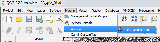
In QGIS, click on Manage and Install Plugins. Search for and install a plugin called Point sampling tool.
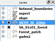
In the QGIS table of contents, check the boxes for the relevant layers only. Start with the SRTM elevation layer and the fine 0.01 degree grid over forest areas.
Under the Plugins menu, click on Analyses and Point sampling tool.
Use point sampling tool to add elevation to the grid file.
- Select the fine forest grid as the layer containing sampling points.
- Select the SRTM elevation data, band 1 raster.
- Specify the output location and file name. Check the box to load the resulting layer once the process is complete. Then click OK.
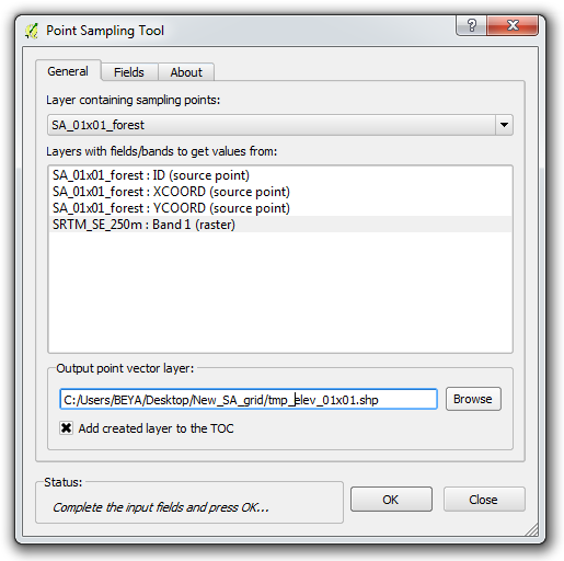
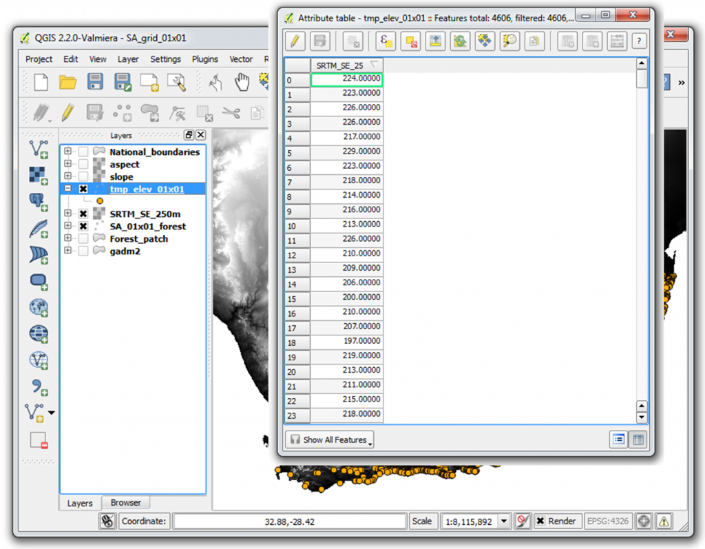
The resulting shapefile contains the elevation at each point.
Repeat the process for slope and aspect. There should be separate shapefiles for elevation, slope and aspect.
To consolidate the elevation, slope and aspect data with the main forest grid, click on the Vector menu and select Data Management Tools, then Join attributes by location.
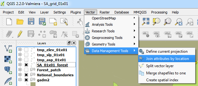
Start by adding elevation data.
- Select the forest grid (with coordinates) for the target vector layer.
- Select the elevation points as the vector layer to join.
- Take attributes of the first located feature.
- Specify the output location and file name. Keep only matching records. Then click OK.
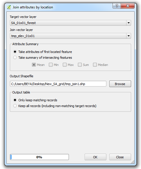
Repeat the process for slope and aspect data, but remember to change the target vector file to the most recent join.
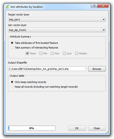
The intermediary elevation, slope and aspect point files and the first two spatial joins are temporary files that can be deleted once the final shapefile is produced. The final join should have a clear file name consistent with the other Collect Earth survey files (no spaces, alpha-numeric characters only).\
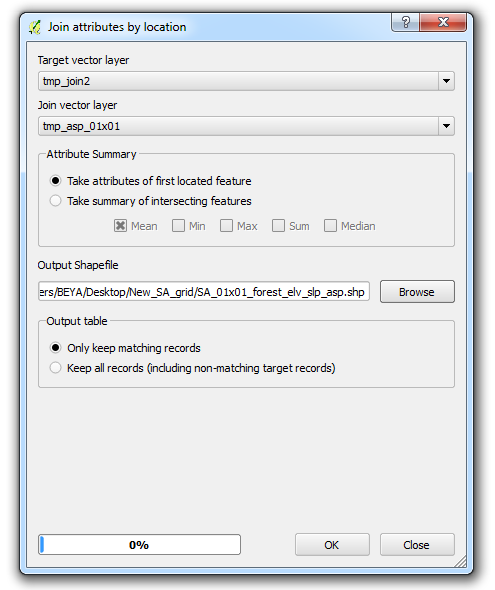
After consolidating elevation, slope and aspect data with the main forest grid, right-click on the layer and review the data attributes table to confirm that the process has been completed properly.
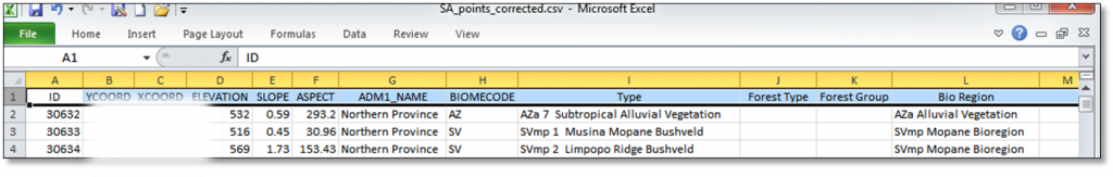
Collect Earth uses grids in csv format with six basic attributes in a particular order:
- plot ID number
- latitude (y coordinate)
- longitude (x coordinate)
- elevation
- slope(x coordinate)
- aspect
Collect Earth South Africa draws upon several additional attributes. Again, the order of the columns is important for compatibility, but the columns can be empty if such data is not available or up-to-date:
- adm1 name
- biome code
- type
- forest type
- forest group
- bio region
The final shapefile produced is comprised of six separate files. Open the DBF file in Libre Office or Microsoft Word.
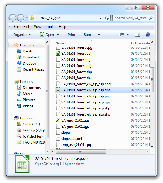
Remove all &, ‘, “ and other symbols that are not alpha-numeric characters from the headers and all of the rows in the spreadsheet. Adjust the order and the names of columns. Note that the order of the coordinates must be reversed so that the y coordinate (latitude) precedes the x coordinate (longitude). Save the file as a csv.
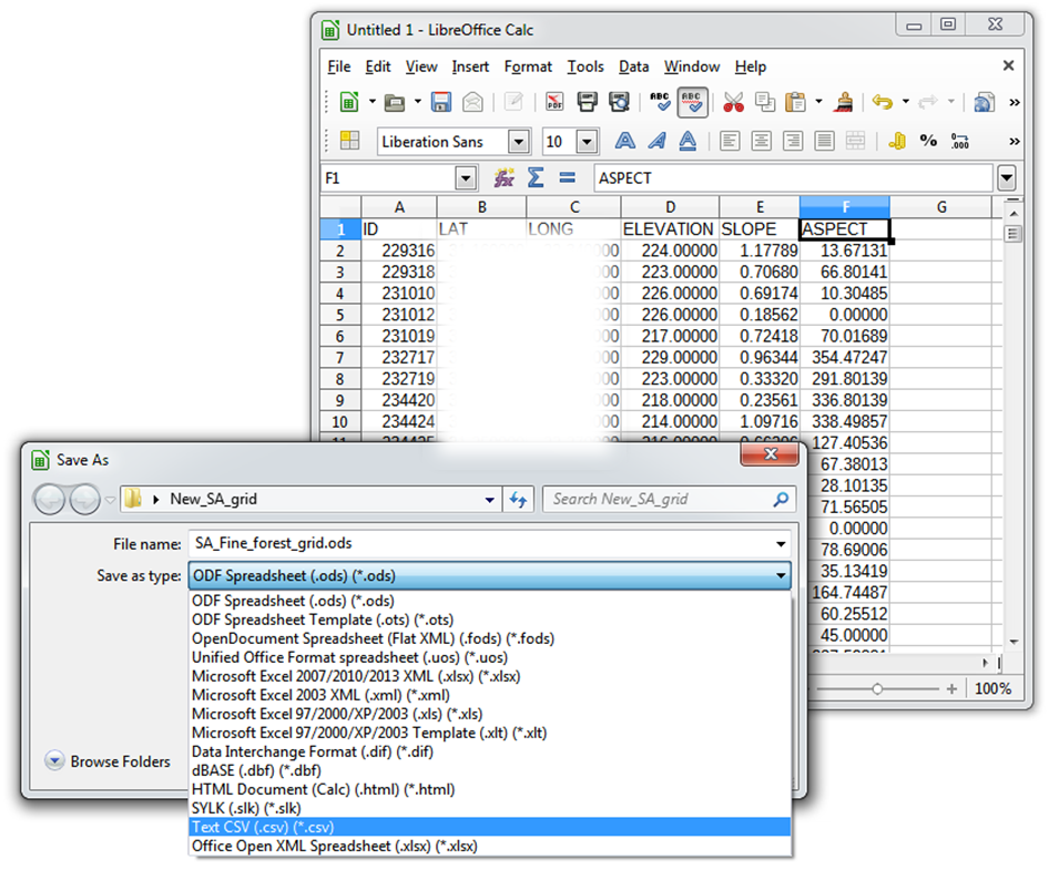
If supplementary data is not available for the extra columns (province name, biome code, biome type, forest type, forest group and bioregion in this case), the column headers still must be added, but the rows beneath the header can remain blank.